eCSE03-11: local excitement in CP2K (12 months)

http://www.cp2k.org

Main focus: excited states using linear response TDDFPT, and support of hybrid functionals

Sergey Chulkov, Matt Watkins

School of Mathematics and Physics, University of Lincoln, UK

Lincoln is here

Why are we interested in excited states?

• Photochemistry
  • Photocatalysis
• Energy conversion
  • Solar cells
• Spectroscopy

TDDFT

DFT normally thought of as ground state theory.

But, time dependent version actually has quite long history - it didn't really achieve prominence until Casida's reformulation caught on with Quantum Chemistry community.

Dynamic polarizabilities and excitation spectra from a molecular implementation of time‐dependent density‐functional response theory: N2 as a case study, Christine Jamorski, Mark E. Casida and Dennis R. Salahub, J. Chem. Phys. 104, 5134 (1996)

TDDFT solves the time-dependent Kohn-Sham equations. If the system is responding to the perturbation caused by an electric field, then we can extract the optical properties of the system from the response.

Two main methods to determine this response by solving the TDKS equations

• Linear-response Time Dependent Density Functional Perturbation Theory
• Real time propagation

both methods are available in CP2K.

Runge-Gross theorem

The time-dependent counterparts of the Hohenberg-Kohn theorems is the Runge-Gross theorem

By solving the Schrodinger equation for external potentials $V(t)$ and a fixed initial state we can map an external potential to a charge density

$$ G:v(r,t) \rightarrow n(r,t) $$
the Runge-Gross theorem says that this map is invertible (subject to some conditions that are still being refined):

$$ G^{-1}:n(r,t) \rightarrow v(r,t) + C(t) $$

This means that the density of a time-dependent system determines the time-dependent potential, which in turn determines the time-dependent wavefunction: every physically meaningful property can be regarded as a functional of the density.

(we ignore the purely time-dependent function $C(t)$ as it only introduces a physically unimportant phase-factor $\bar{\Psi}(t) = e^{-i \alpha (t)}\Psi(t)$, where $\dot{\alpha}(t) = C(t)$)

Action functional

The equivalent of the energy functional $E[n]$ of a time-independent system for a time-dependent system is

$$ A[n] = \int_{t_0}^{t_1} \text{d}t \left< \Psi[n](t)\big{|} i\frac{\partial}{\partial t} - H(t) \big{|} \Psi[n](t) \right> $$

The exact time-dependent density is a stationary point of this functional

$$ \frac{\partial A}{\partial n(t)} = 0 $$

How to approximate $A_{XC}[n]$?

Just use the same functional of the density as ground state DFT, but use the density at the current time.

Adiabatic local density approximation (ALDA)

if we don't know much about the exchange correlation functional, we know even less about the time dependent action functional.

The normal approach is to use the ALDA

$$ f_{xc}(r,t; r',t') ≈ δ(t − t')\frac{\delta^2 E_{xc}^{LSDA/GGA}[n]}{ \delta n(r,t)\delta n(r',t')}_{n(r,t)=n^{(0)}(r,t)} $$

it is memoryless - response doesn't depend on history, and local.

We use a standard density functional evaluated with the current ground state density.

Almost universal approach at the moment - some research on current / memory functionals

Time dependent Kohn-Sham equations

at this point we can introduce one-electron orbitals and obtain the equivalent of the KS-DFT equations.

The time-dependent density is

$$ n(r,t) = \sum_{i \in HOMOs}\psi_i(r,t)^* \psi_i (r,t) $$

we find the appropriate density by the condition

$$ \frac{\delta A}{\delta n(t)} = 0 $$

and after a bit of work we get

$$ \big{[} -\frac{1}{2}\nabla^2 + v_s[n](r,t) \big{]} \psi_i(t) = i \frac{\partial \psi_i(t)}{\partial t} $$

with the effective potential

$$ v_s[n](r,t) = \int_r' \text{d}r'\frac{n(r',t)}{\mid r' - r\mid} + v(r,t)+ \frac{\delta A_{XC}[n]}{\delta n} $$

all that needs to be done is to solve the equations given a set $\psi_i(r,t_0)$.

Two main methods to solve the TDKS equations

Linear-response Time Dependent Density Functional Perturbation Theory

Real time propagation

both methods are available in CP2K.

Matrix equations

Skipping quite a bit -

we introduce basis functions

and work in a linear response regime

because the response orbitals should be orthogonal to the ground state orbitals we expand them as a linear combination of LUMOs

$$ \psi_{i, \sigma}^{(\pm)}(r) = \sum_{j \in LUMOs} c_{i,j, \sigma}\psi_{j,\sigma} (r) $$

Electron hole pairs

The transition density is a linear combination of $\color{red}{electron}-\color{blue}{hole}$ pairs

\begin{gather*} \left ( \color{blue}{\psi_{j,\sigma}^*} (r) \color{red}{\psi_{j,\sigma}^{(-)}(r)} + \color{red}{\psi_{j,\sigma}^{(-)*}(r)}\color{blue}{ \psi_{j,\sigma}(r)} \right) e^{-i \omega t} \end{gather*}

in the ground state the $\psi_{j,\sigma}$ function would be fully occupied, but here density has be transferred to $\psi_{j,\sigma}^{(-)}(r)$ .

$\color{blue}{\psi_{j,\sigma} (r) }$ is the hole, $\color{red}{\psi_{j,\sigma}^{(-)}(r)}$ the electron.

The sum over all the HOMOs allows the hole to relax by mixing in other occupied orbitals.

Each of the terms in the sum are single determinant excitation in Quantum Chemical language.

Typical transitions will be dominated by a single determinant - mixing of others gives orbital relaxation.

Using the same basis of contracted Gaussian functions as for the ground state, we finally get

\begin{gather*} \sum_{\nu} \big{(} \mathbf{F_{\nu \mu \sigma}} c_{\mu j \sigma}^{(-)} - \mathbf{S_{\nu \mu} c_{\mu j \sigma}^{(-)} \epsilon_{j \sigma}}\big{)} + \\ \sum_{\nu} \sum_{\gamma} \big{(} \delta_{\mu \gamma} - \sum_k \sum_{\delta} \mathbf{S_{\mu \delta }} c_{\delta k \sigma}^{(0)} c_{\gamma k \sigma}^{(0)} \big{)} \mathbf{K_{\gamma \nu \sigma}} c_{\nu j \sigma}^{(0)} = \omega \sum \mathbf{S_{\nu \mu \sigma}}c_{\mu j \sigma}^{(-)} \end{gather*}

where

$$ \mathbf{F_{\nu \mu \sigma}} = \big{<} \phi_{\nu} \big{|} H^{(0)}_{\sigma}\big{|} \phi_{\mu} \big{>} $$

is the ground state KS matrix

and

$$ \mathbf{K_{\nu \mu \sigma}} = \big{<} \phi_{\nu} \big{|} \sum_{\tau=\alpha, \beta} \big{[} \int_{r'} \text{d}r' \frac{n_{j, \tau}^{(1)} (r')}{\mid r' - r\mid} + f_{XC,\sigma,\tau} (r,r';\pm \omega)) n_{j, \tau}^{(1)} (r') \big{]} \big{|} \phi_{\mu} \big{>} $$

is the TDDFPT Kernel for a semi-local density function.

For hybrid functionals we add in an extra coulomb type term that comes from the response of the exact exchange part of the functional.

These look horrible, but are an Eigenvalue problem that can be solved to give eigenvalues and eigenvectors corresponding to excitations of the system.

Tamm-Dancoff approximation

only the Tamm-Dancoff approximation to TDDFT is implemented in CP2K at the moment.

In this approximation $\phi^{(+)}_{j\sigma} (r) = 0$ and the equations simplify and become Hermitian.

Hybrid functionals

For hybrid functionals we add in an extra term that comes from the response of the exact exchange part of the functional.

With hybrid density functionals the original action functional becomes a mixture of the TDDFT outlined above and TDHF.

• The coulomb interaction in standard functionals actually becomes an exchange like term, dependent on wavefunction overlap between the electron and hole.

\begin{gather} \mathbf{K_{\nu \mu \sigma}} = \big{<} \phi_{\nu} \big{|} \sum_{\tau=\alpha, \beta} \big{[} \color{red}{\int_{r'} \text{d}r' \frac{n_{j, \tau}^{(1)} (r')}{\mid r' - r\mid}} + f_{XC,\sigma,\tau} (r,r';\pm \omega)) n_{j, \tau}^{(1)} (r') \big{]} \big{|} \phi_{\mu} \big{>} \end{gather}\begin{gather*} \color{red}{ n_{j, \sigma}^{(1)} (r) = \sum_{j \in HOMOs} \left ( \psi_{j,\sigma}^* (r) \psi_{j,\sigma}^{(-)} (r) \right) + \left ( + \psi_{j,\sigma}^{(-)*}(r) \psi_{j,\sigma}(r) \right) } \end{gather*}

Semi-local functionals have incorrect long-range behaviour because of this - well known underestimation of charge transfer states.

• the exact exchange energy term in the ground state functional becomes a coulomb type interaction between the electron and hole density for each excitation.

\begin{gather} \mathbf{K_{\nu \mu \sigma}} = \big{<} \phi_{\nu} \big{|} \sum_{\tau=\alpha, \beta} \big{[} \color{green} { c_{HF} \frac{K(r,r')}{ {\mid r' - r\mid}}} + \color{red}{ \int_{r'} \text{d}r' \frac{n_{j, \tau}^{(1)} (r')}{\mid r' - r\mid}} + \color{green}{(1-c_{HF})} f_{XC,\sigma,\tau} (r,r';\pm \omega)) n_{j, \tau}^{(1)} (r') \big{]} \big{|} \phi_{\mu} \big{>} \end{gather}

where the symbolic $\color{green}{K(r,r')}$ operator exchanges electrons, like in HF theory. In this case operating on an exchange type term, it gives an electron-hole coulomb interaction. Symbollically, terms of the form:

$$ \color{green}{ \big<\psi_{HOMOS} (r) \psi_{HOMOS} (r) \big| { \frac{1}{\mid r' - r\mid}} \big| \psi_{LUMOS} (r') \psi_{LUMOS} (r') \big> } $$

Note this is like a coloumb interaction screened by an effective dielectric function equal to $\color{green}{c_{HF}^{-1}}$.

Implementation

We followed the original implementation of TDDFPT for semi-local functionals within CP2K (Thomas Chaissang's PhD thesis). But, ended up with complete rewrite.

Currently separate implementation (TDDFPT2). Original is deprecated, and will be removed in future.

• It is activated within the &PROPERTIES section of &FORCE_EVAL - so can be used within MD or MC or single point calcs etc.

• XC section is inherited from the ground state calc - needs weak smoothing SPLINE2_SMOOTH on the XC gradients.

Uses a standard block Davidson algorithm for iterative diagonalization of excited states.

• Semi-local DFT terms are calculated on realspace multigrids

\begin{gather} \mathbf{K_{\nu \mu \sigma}} = \big{<} \phi_{\nu} \big{|} \sum_{\tau=\alpha, \beta} \big{[} \color{red}{\int_{r'} \text{d}r' \frac{n_{j, \tau}^{(1)} (r')}{\mid r' - r\mid}} + f_{XC,\sigma,\tau} (r,r';\pm \omega)) n_{j, \tau}^{(1)} (r') \big{]} \big{|} \phi_{\mu} \big{>} \end{gather}

• Because of the exchange, this is not possible for the added exact exchange term with iterative diagonalisation: Hybrid term is calculated analytically using the existing hybrid functional routines in CP2K
  • including access to fast methods like ADMM. (x1000 speed up for some basis sets)

• Oscillator strengths calculated using the velocity operator form of the dipole interaction - which can be translated into a term related to the derivative of the overlap matrix (similar to force calculation in local basis set codes).

  • should be valid in periodic systems (scarcely tested though)
  • might be subject to noise in some cases

• Extra layer of parallelism over excitations is available, but may have too high initial communication overhead to be viable - to be continued...

Input files

Here is an example input for formaldehyde (CH$_2$O)

The TDDFPT calculation is activated by the &PROPERITIES section. And doesn't need to much messing with.

This needs a very up-to-date version of CP2K (like the default on ARCHER!)

Here we calculate 3 excited states.

&GLOBAL PROJECT ch2o_pbe0_rks_s_tddfpt RUN_TYPE energy PRINT_LEVEL medium &END GLOBAL

&FORCE_EVAL METHOD Quickstep

&PROPERTIES &TDDFPT NSTATES 3 # number of excited states MAX_ITER 10 # maximum number of Davidson iterations CONVERGENCE [eV] 1.0e-3 # convergence on maximum energy change between iterations
&MGRID CUTOFF 200 # separate cutoff for TDDFPT calc &END &END TDDFPT &END PROPERTIES

&DFT BASIS_SET_FILE_NAME GTH_BASIS_SETS POTENTIAL_FILE_NAME POTENTIAL &MGRID CUTOFF 400 &END MGRID &QS METHOD gpw &END QS &SCF MAX_SCF 30 EPS_SCF 1e-7 SCF_GUESS atomic &END SCF &POISSON PERIODIC none POISSON_SOLVER wavelet &END POISSON &XC &XC_FUNCTIONAL pbe0 &END XC_FUNCTIONAL &XC_GRID XC_DERIV SPLINE2_SMOOTH # this is needed for the 2nd derivatives of the XC functional &END XC_GRID &HF &SCREENING EPS_SCHWARZ 1.0E-10 &END SCREENING &END HF &END XC &END DFT &SUBSYS &TOPOLOGY &CENTER_COORDINATES &END CENTER_COORDINATES &END TOPOLOGY &CELL ABC 9.0 9.0 9.0 PERIODIC NONE &END CELL &COORD O 0.9588431900 1.1234806613 1.8643358699 C 1.0045827842 1.0372747429 0.6713062328 H 1.0304990091 1.9328340670 0.0202209074 H 1.0234151411 0.0574091066 0.1554705073 &END COORD &KIND O BASIS_SET aug-TZV2P-GTH POTENTIAL GTH-PBE-q6 &END KIND &KIND C BASIS_SET aug-TZV2P-GTH POTENTIAL GTH-PBE-q4 &END KIND &KIND H BASIS_SET aug-TZV2P-GTH POTENTIAL GTH-PBE-q1 &END KIND &END SUBSYS &END FORCE_EVAL
</code>

After the ground state calculation you should see something like

TDDFPT WAVEFUNCTION OPTIMIZATION Step Time Convergence Conv. states 1 1.3 1.1524E-02 0 2 1.4 1.1928E-03 0 3 1.4 1.0624E-03 2 4 1.4 4.0385E-05 2 5 1.3 5.0590E-07 3 Restart Davidson iterations 6 1.3 8.9465E-05 1 7 1.3 2.1614E-09 3

and when it converges

*** TDDFPT run converged in 7 iteration(s) *** R-TDDFPT states of multiplicity 1 State Excitation Transition dipole (a.u.) Oscillator number energy (eV) x y z strength (a.u.) TDDFPT| 1 3.83726 -0.0000 0.0000 -0.0000 0.00000 TDDFPT| 2 5.84022 0.0008 0.3265 -0.0000 0.01526 TDDFPT| 3 6.59404 0.0338 -0.0001 0.3225 0.01699 Excitation analysis State Occupied Virtual Excitation number orbital orbital amplitude 1 6 7 -0.999718 2 6 8 -0.997564 3 6 9 -0.996738 6 16 -0.052845

The 'occupied' and 'virtual' orbital sections show which are the dominant contributors to a transition

Visualisation

orbitals can be viewed by

• outputing MO cubes

&DFT &PRINT &MO_CUBES STRIDE 1 # for accurate visualisation NHOMO x NLUMO y &END &END &END

• outputing the wavefunctions in MOLDEN format (new!) feature
  • VMD can process the single MOLDEN wavefunction file to view orbitals

&SCF &PRINT &MOS_MOLDEN &END &END &END

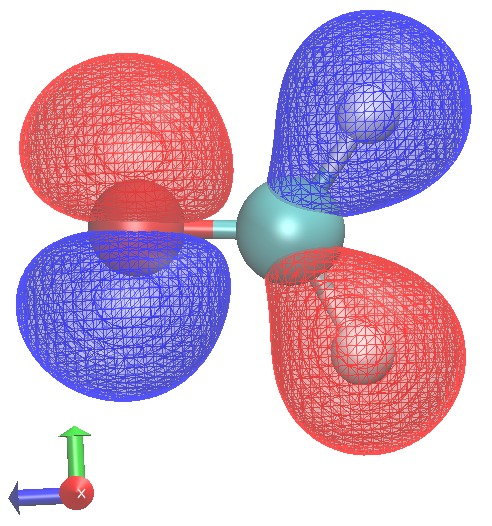HOMO to LUMO transition has no oscillator stength (not totally symmetric under 'multiplication' with 'x,y or z')

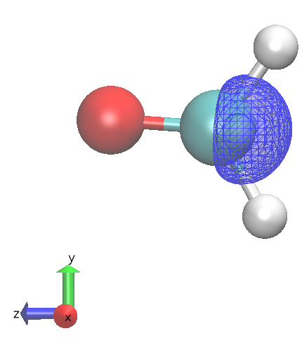HOMO to LUMO + 1 allowed

Linear response summary

• gives electron transitions and detailed information on the types of transition
• cost will depend on system size, but increase linearly with the number of excited states that you want to calculate
• supports calculations using hybrid functionals and the ADMM approximation
• current implementation is very much in beta, but is being actively developed.
• nearly production ready, needs final testing and refining - is available in trunk via sourceforge or github

Excited state forces

Currently only energies with LR-TDDFTPT.

Two options

1. Ehrenfest dynamics - see Samuel Andermatt, Jinwoong Cha, Florian Schiffmann, and Joost VandeVondele, J. Chem. Theory Comput., 2016, 12, pp 3214–3227 DOI: 10.1021/acs.jctc.6b00398

2. Maximum Overlap Method - systems constrained to single excited state determinant calculated self consistently (delta-SCF) method - see Andrew T. B. Gilbert, Nicholas A. Besley and Peter M. W. Gill, J. Phys. Chem. A, 2008, 112 (50), pp 13164–13171 DOI: 10.1021/jp801738f

Maximum overlap method

By intitially occupying a LUMO + x and deoccupying a HOMO + y orbital we can build an excited state determinant.

During the SCF cycles we calculate the projection of the new atomic orbitals onto those of the previous cycle

$$ \mathbf{O} = (\mathbf{C^{old}}) \mathbf{SC^{new}} $$

When building the new density matrix, instead of following the Aufbau Principle, we occupy the $nelectron$ states most like the $nelectron$ orbitals occcupied in the previous cycle.

This is performed self consistently. When self-consistent, forces and other properties can be calculated using normal ground state routines.

Examples in regtest-mom-[12]

&SCF MAX_SCF 40 EPS_SCF 1e-6 SCF_GUESS restart ADDED_MOS 5 &MIXING ALPHA 0.2 &END MIXING &MOM on DEOCC_ALPHA 3 OCC_ALPHA 5 &END MOM &END SCF

MOM is activated in the SCF section.

• Must use traditional diagonalisation rather than OT
• Must have some ADDED_MOS
• Specify orbitals to occupy and deoccupy to make initial state

Thanks To

• Joost VondeVondele (?)
• Juerg Hutter (University of Zurich)
• Alex Shluger (UCL)
• CP2K developers
• Iain, EPCC, ARCHER